The content of this website contains the personal opinions of the members of group 12 only,
and is not the opinion of the University of Southampton or the National Oceanography Centre
Southampton.
Falmouth 2017 - Group 12 7TITLE


Offshore
Discussion
Physical
Chemical
Station 8
The salinity remains constant during deployment 1 at a value of 35.4. However, during deployment 2, there is a spike in salinity at around 15 m from 35.4 to 36.4 this is most likely due to the CTD.
As the depth decreases, the temperature also decreases, this is what is expected from this type of profile.
There is a thermocline at 15 m but the temperature carries on decreasing until around 40 m

Station 9
The salinity stays constant throughout the water column, this is because the profile was taken out to sea, where there are not any sources of freshwater
The temperature profile shows that temperature decreases with depth, this is what was expected.
There is a thermocline at around 18 m and extends to 40 m

Station 10
The salinity at station 10 remained constant through the water column, it remains at 35.4 psu
The temperature decreases with depth in the surface waters the temperature is 16°C but at 50 m depth, the temperature is 12.5 °C.
There is a thermocline between 37 and 40 m

Station 11
At station 11, a yo-yo profile was performed, this is where the CTD was lowered multiple times and this is to collect data on the wave structure.
The salinity remains constant with a very small variation throughout the water column during all deployments.
The temperature decreases with depth and all of the CTD deployments follow this trend.
There is a thermocline at 35 m


Phosphate
- Surface concentration stays low from 10:00 – 14:00 this would be due to a high concentration of phytoplankton in the surface waters utilizing most of the bioavailable phosphate.
- 14:00 there is an increase in concentration of phosphate in the surface waters, could be due to CDOM dissolving back into the water, which would increase the phosphate concentration.
- The levels are what were expected between 10:00 and 14:00
- The chlorophyll levels remain low in the surface water, but at the DCM the chlorophyll concentration increases with the phosphate concentration.
Terramare nutrient plots (Time Series)
Biological
Nitrate
- Not as expected, surface water has a higher concentration than the water at the DCM, only at 13:00 where the surface has a lower conc than at the DCM.
- The surface chlorophyll remains constant at the surface and the 30 m chlorophyll concentration mirrors the increase in nitrate at around 13:00
Silicate
- Surface concentration remains lower than the concentration at 30 meters – which is expected
- Steady increase in silicate concentration at the DCM between 11:00 and 14:00 could be due to an increase in CDOM in the water and silicate dissolving back into the water.
- The surface chlorophyll concentration remains the same over the time period, but the increase in chlorophyll concentration occurs at 13:00 and the increase in silicate is around 14:00 showing that chlorophyll and silicate levels may not be directly linked ?


Describing biological data – Offshore
Phytoplankton Offshore abundance:


Station8
2m: species richness is 4 and species evenness is 0.676. Most abundant species: Rhizosolenia setigera with 69% of abundance and 92% of abundance accounted for the genus Rhizosolenia spp. Total phytoplankton count is 13 specimens (very low count so not very reliable results).
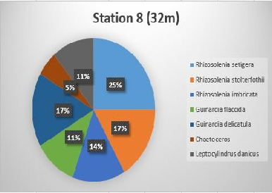
32m: species richness is 9 and species evenness is 1.36. Most abundant species: Rhizosolenia setigera with 20% of abundance and 45% of abundance accounted for the genus Rhizosolenia spp. Total phytoplankton count is 44 specimens.
Station 9
2m: species richness is 4 and species evenness is 1.0. Most abundant species is Rhizosolenia alata with 40% of abundance and 60% of abundance accounted for the genus Rhizosolenia spp. Total phytoplankton count is 5 specimens (very low count so not very reliable results).
32m: species richness is 8 and species evenness is 0.711. 53% of abundance accounted for the genus Chaetoceros spp. Total phytoplankton count is 103 specimens.
Station 10
2m: species richness is 7 and species evenness is 0.917. Most abundant species: Rhizosolenia setigera with 33% of abundance. Total phytoplankton count is 52 specimens.
30m: species richness is 11 and species evenness is 0.930. Most abundant species: Rhizosolenia setigera with 20% of abundance. 33% of abundance accounted for the genus Rhizosolenia spp. Total phytoplankton count is 85 specimens.
Station 11
2m: species richness is 7 and species evenness is 0.980. 25% of abundance is accounted for the genus Chaetoceros spp. Total phytoplankton count is 8 specimens (very low so not very reliable results).
30m: species richness is 5 and species evenness is 0.917. Most abundant species: Ceratium tripos with 43% of abundance and 57% of abundance accounted for the genus Ceratium spp. Total phytoplankton count is 7 specimens (very low so not very reliable results).
Station 12
2m: species richness is 5 and species evenness is 0.785. Most abundant species: Rhizosolenia setigera with 54% of abundance. Total phytoplankton count is 13 specimens (very low so not very reliable results).
30m: species richness is 6 and species evenness is 0.904. 35% of abundance accounted for dinoflagellates. Total phytoplankton count is 17 specimens (very low so not very reliable results).


Figure 1: Contour plot of temperature changes with depth and time measured with a CTD 05.07.2017 between 09:20 and 14:38 UTC at a location lat 50˚05.842 and lon 004˚52.122.
Figure 2: Contour plot of temperature changes with depth and time measured with a CTD 05.07.2017 between 09:20 and 14:38 UTC at the location lat 50˚05.842 and lon 004˚52.122.
Description
Figure 1 shows temperature contours close together around 10-15 meters depth in the beginning of the time series. After 10:30 UTC until around 14:00 UTC the contours are spreading out before aligning again in the end of the time series. The surface contours until around 10 meters are changing from vertical to horizontal throughout the time series. Below 15 meters the contours are mostly horizontal and around 14:00-15:00 UTC the contours are aligning vertically around 15-25 meters.
Figure 2 shows an overall low chlorophyll concentration in the first half of the time series. Around 13:00 UTC the concentration increases rapidly showing a peak around 30-35 meters as well as a smaller peak around 13 meters in the end of the time series from 14:00 to 16:00 UTC.
TDS plots
| Background |
| Gallery |
| Results |
| Discussion |
| Results |
| Discussion |
| Results |
| Discussion |